
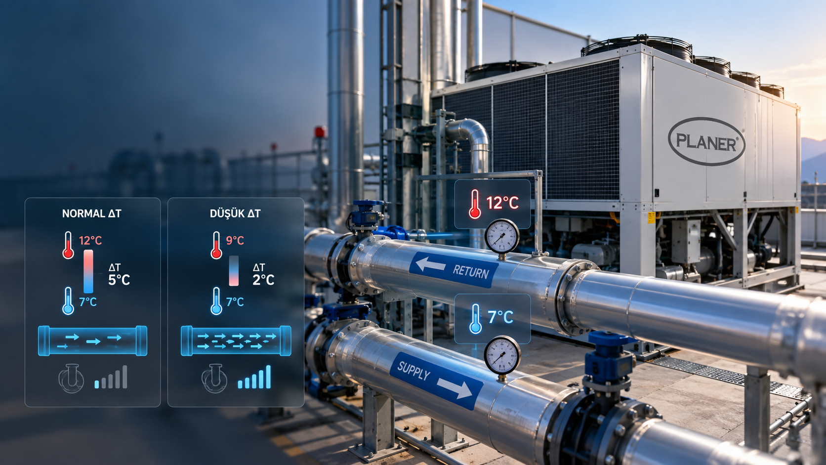
A chiller's delta-T reports the hydraulic health of a chilled-water circuit in a single number: how much heat the plant is carrying, how much electricity the pump is drawing and whether the compressors are running steadily. It is also where a familiar site picture begins: ΔT sits well below its design value, the flow rate climbs, pump energy rises — and the process still will not cool. This set of symptoms goes by the name low delta-T syndrome, and its source usually lies not inside the chiller but in the circuit through which the water travels around the plant. In this article we cover the ΔT calculation, where the design value comes from, the seven typical causes of low ΔT, what it costs, how to measure it in the field, and the role of the buffer tank.
What chiller ΔT is and how it is calculated
ΔT (delta-T) is the difference between the inlet and outlet water temperatures across the chiller evaporator; the inlet is the water returning from the process, the outlet the water sent back to it. If water returns from the process at 12 °C and leaves the chiller at 7 °C, ΔT is 5 °C. That difference acquires its meaning only alongside the flow rate; the heat carried by the water is the product of flow rate and temperature difference:
Q (kW) = flow rate (m³/h) x 1.163 x ΔT (K)
The 1.163 here is not an arbitrary coefficient but the physics of water itself. Raising the temperature of one cubic metre of water by 1 K takes roughly 4,186 kJ of energy; since 1 kWh is 3,600 kJ, that energy amounts to 1.163 kWh. The unit of the coefficient is therefore kWh/(m³·K); give the flow rate in cubic metres per hour and the product reads directly in kW.
The formula works in both directions. In design it yields the flow rate: carrying a 100 kW load at a ΔT of 5 °C calls for 100 / (1.163 x 5) = 17.2 m³/h of water. In diagnosis the third value is calculated from two measured ones; in the same circuit, at a flow rate of 17.2 m³/h but a ΔT of 2.5 °C, the heat being carried is 17.2 x 1.163 x 2.5 = 50 kW. Whatever capacity the chiller's nameplate states, that is the heat actually being drawn from the plant at that moment.
The design ΔT is a chosen value; the ΔT measured in operation is not a setting but a result that establishes itself according to the real load, the circulating flow rate and the condition of the heat-transfer surfaces. Measured ΔT is the cheapest diagnostic indicator there is: a pair of thermometers is enough to obtain it.
Why a 5 °C ΔT? Where the design value comes from
The ΔT of around 5 °C common in process cooling is not a constant of nature but a balance struck between two cost items; the 12/7 °C regime is the classic expression of that choice. Carrying the same load at a ΔT of 10 °C halves the flow rate, to roughly 8.6 m³/h; three constraints explain why a high ΔT is nevertheless not always preferred:
- The process side: with the outlet temperature fixed, a larger ΔT raises the mean temperature of the water reaching the mould, the jackets and the process exchangers; rejecting the same heat then demands more transfer surface, and in processes that require a narrow band, product quality is affected.
- The evaporator side: as the flow rate falls, velocity and turbulence drop and the heat-transfer coefficient declines. Every exchanger has a flow range specified by its manufacturer; going outside it brings freezing and fouling risks.
- The control side: a small flow rate means the water in the circuit takes longer to complete a lap; the water volume may be unchanged, but the rate at which heat is carried falls, dead time lengthens, and temperature swings more quickly on sudden load changes.
What matters is not the number chosen but consistency: chiller capacity, pump, pipe diameters, valves and buffer tank volume must all be sized to the same ΔT. A high ΔT does bring one gain, in free cooling: as the return water grows warmer, its difference from the outside air widens and the free cooling window broadens.
What low delta-T syndrome is
Low delta-T syndrome is a circuit's persistent failure to reach its design ΔT: even with the plant under load, the measured ΔT stays well below the design figure while the circulating flow rate equals or exceeds the design flow. The term is established in the operating practice of district cooling and large chilled-water systems; it is called a syndrome because what is present is not a single faulty part but a set of symptoms arising from the system as a whole:
- ΔT is well below design and does not improve as the load rises; more often than not it narrows further.
- The pump runs at full speed, frequently above the design flow rate, while some of the compressor stages never cut in, or stop shortly after doing so.
- The chiller holds its outlet water temperature comfortably; even so, the process does not come down to its target temperature.
The chiller does not set ΔT, but it does respond to it. Since the load it sees is the product of flow rate and ΔT, when the return water arrives colder than it should, less capacity is enough to hold the outlet water at setpoint; the machine reads this as "the load has dropped" and unloads a stage. On units that stage capacity directly from return water temperature, the same outcome follows even more directly. Yet the heat from the process is exactly where it was: while the machine sheds load, the plant heats up, and the result is lost production. Circulating still more water in response to the complaint only drives ΔT lower, as the equation requires.
Seven typical causes of low ΔT
Different as the causes look, they meet on common ground: each either sends water round the circuit without picking up heat, or reduces the heat that could be picked up.
- Open bypass lines and three-way valves: a bypass someone forgot to close, or a three-way valve that mixes, blends cold water that has never passed through a consumer into the return line and pulls the return temperature down. The same effect appears at decouplers where the primary flow exceeds the secondary flow: the surplus primary water crosses from supply to return through the balance pipe.
- Fouled heat-transfer surfaces: the scale, sediment and biofilm accumulating in the evaporator, in the process exchanger or in the mould channels behave like insulation; the water picks up less heat and returns colder than it should.
- Excessive pump flow: an oversized, unbalanced or fixed-speed pump pushes more water into the circuit than the design calls for. Since the load has not changed, the only outcome of the surplus flow is that ΔT is divided up; it is one of the causes met most often in circuits without balancing valves.
- Incorrect sensor location and calibration: ΔT is a differential measurement; across a 5 °C difference, a 0.5 °C deviation between two sensors misrepresents the calculated ΔT — and therefore the calculated heat — by 10% in theory. A sensor not seated fully in its thermowell, or sitting too close to a mixing point, can make a picture that does not exist look real.
- Failing to account for glycol: the volumetric heat capacity of a water-glycol mixture, that is density times specific heat, is below that of pure water; carrying the same load therefore requires a higher flow rate, and the 1.163 coefficient valid for pure water loses its validity in the mixture. Multiplying ΔT by 1.163 in a glycol circuit overstates the heat being carried; a circuit selected on that basis, with too little flow, shows up in the field as a capacity shortfall. The mechanism that actually produces the low ΔT, though, is viscosity: as viscosity rises, heat transfer in the exchanger weakens and the water returns from the process colder than it should; moreover the pump, upsized for the glycol, more often than not pushes more water into the circuit than the design calls for. The size of the effect depends on the mixture ratio and the temperature, and should be read from the manufacturer's or supplier's property tables.
- A real load below the design load: if the heat coming from the process really has fallen, a low ΔT is not a fault but the natural consequence of the equation. In a constant-flow system, once this becomes permanent the problem lies not in the circuit but in the sizing and the control strategy.
- Air trapped in the circuit: air collecting at high points throttles the flow in some branches and takes part of the exchanger surface out of service; the symptoms are erratic flow, pump noise and fluctuating temperatures.
In the field these causes are usually found stacked on top of one another; the list has to be narrowed down by measurement.
What low ΔT costs the plant
The first and most striking item is pump energy. If ΔT halves, carrying the same load requires the flow rate to double; on a fixed system curve, pressure loss varies with the square of flow and shaft power with the cube, so in theory the pressure loss rises roughly fourfold and the pump power roughly eightfold. In a real plant, static head, valve characteristics and the motor efficiency curve soften that ratio — but the direction does not change.
The second is unusable capacity: the heat that can be carried is limited by the product of flow rate and ΔT, and once the pump can push no more water the plant cannot make full use of its installed capacity. The third is mechanical wear; stages fail to come on or shut down again shortly after, start-stop counts rise, and oil return and contactor life are put under strain. The fourth is lost free cooling: because the coil sits on the return line, cold return water narrows the difference against the outside air and free cooling hours fall.
The fifth is the most expensive of all: the picture is mistaken for a capacity shortfall and a new unit is bought. Since the circuit is unchanged, the problem persists, and this time the plant runs a larger machine at a lower load.
Field measurement and verification
An argument about low ΔT is settled by measurement, not by guesswork; the diagnosis starts not with the instantaneous value on the panel display but with supply, return and flow rate measured independently and simultaneously. The following sequence can be followed to narrow the diagnosis down with the records of a single shift:
- Timing the measurement to a period when the process is at full load; a low ΔT read at low load is normal and carries no diagnostic value.
- Reading supply and return temperatures simultaneously with two matched probes on the same calibrated instrument; if a single probe has to be used, the two points must be measured one after the other within a short window in which the load stays constant, because across a difference of a few degrees a systematic sensor offset can reverse the result.
- Measuring the flow rate rather than assuming it, with an ultrasonic flow meter on a straight, fully flooded length of pipe, or across a balancing valve.
- Calculating Q from the three measured values and comparing it against the unit's capacity derated to that operating condition — that is, to the water outlet temperature and the outside air temperature of the moment; the electrical power drawn enters this comparison only once it is converted to thermal power via the efficiency, while the compressor current shows whether the stages are loaded.
- Reading the flow direction and temperature of the bypass line and the balance pipe; this check eliminates the mixing-related causes within a few minutes.
- Not settling for a single instantaneous reading; logging supply, return, flow rate and outside air for at least one shift.
This comparison splits the diagnosis in two. If Q is close to the derated capacity, the machine is doing its job; what is depressing ΔT is excess flow, and the pump side is where to look. If Q is markedly below it and the process is still heating up, the heat is not getting into the water; in that case look for fouled surfaces, an open bypass or mixing valves.
How buffer tank volume protects ΔT
A buffer tank does not create ΔT; it is a thermal mass that prevents ΔT from swinging and prevents short cycling, the most damaging consequence of a low ΔT. Sufficient volume stops the return temperature from being thrown about by sudden load changes and lets the stages run for sensible periods.
The volume required derives from the same physics, from the constant 1.163. One cubic metre of water stores 1.163 kWh of energy if it is allowed to swing by 1 degree; accordingly, the volume needed for a stage of P kilowatts to run for at least t minutes is found, in theory, from V = P x (t / 60) / (1.163 x the permitted temperature band). For example, if a 100 kW stage is to run for 5 minutes and the water is not to deviate by more than 2 °C, roughly 3.6 m³ is required in the worst case, with no load at all coming from the process; in a real plant the process heat is also in the circuit, so the formula gives an upper bound.
How the tank is connected matters as much as its volume: it should be piped in series on the return line, with its connections positioned so that they cannot short-circuit. A wrongly connected tank mixes supply with return inside itself and sends the chiller water that is colder still; the plant deepens the problem with the very equipment installed to solve it. A buffer tank will not correct an open bypass or a fouled exchanger; it only softens the symptom. The order is always the same: verify the hydraulics and the heat transfer first, then establish stability with volume.
Design ΔT, the pump, the buffer tank volume and the chiller capacity are not independent decisions; change one and the others must be recalculated. Planer manufactures air-cooled chillers, water-cooled chillers, dry coolers and hybrid chillers from roughly 16 kW up to 1,270 kW, its units using predominantly R407C and, in some models, R134a. To assess the ΔT behaviour of your circuit, or to isolate the source of low delta-T syndrome on site, you can contact Planer's engineering and service team and request an assessment tailored to your plant on the basis of your own measurement records.